My Tiny Renderer (1/?)

Contents
The Bare Minimum⌗
After goofing around for a while, I discovered ssloy/tinyrenderer. This is an outline on how to build a really basic software renderer. However, I quickly realised that a lot of what was being done was rather (intentionally) handwavey for my taste and I decided that I would go about implementing everything in my own uniquely deranged way while documenting the process.
So for the first few articles I will be following the general outline of ssloy/tinyrenderer. My code will inevitably be slightly different from what ssloy came up with. For instance our line drawing algorithms look slightly different, since we took different routes to get there.
After I’m done with implementing all of the techniques mentioned in the tinyrenderer, I will be making a incredibly sharp turn into realtime rendering with this as the basis.
I made basically no changes to the TGA classes that ssloy came up with, since I plan on ditching the TGA format.
The code at this stage of the article can be found here
Bresenham Line Drawing Algorithm⌗
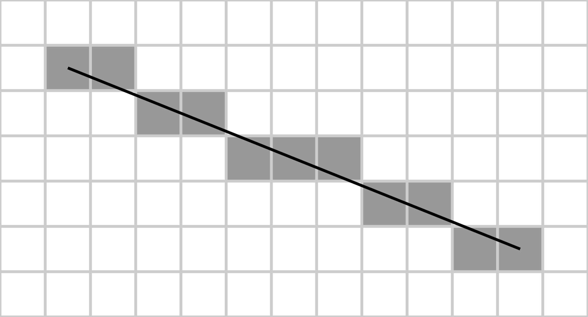
The Bresenham algorithm is specifically designed to work on lines that go downwards (technically its still upwards its just that the way pixel indexing on displays work) with a slope less than 1. This may seem pretty limiting at first but we will extend this method to draw lines at any angle.
Derivation⌗
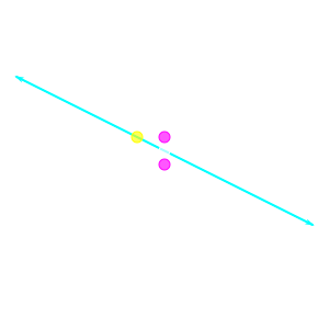
Lets start at \( (x_0, y_0) \) such that \(f(x_0, y_0) = 0 \) and since A, B and C are all integers in the line equation of our choice (they are calculated using start and end point using slopes and so on, you get the idea), so is \(x_0\) and \(y_0\) and is represented by the yellow dot. The intersection of the integral grid lines represent the pixels on the screen.
We move to the right in discrete steps incrementing the value of x. Now we need to decide whether we should colour \((x_0 + 1, y_0)\) or \((x_0 + 1, y_0 + 1)\) we do not need to consider the 8 total vertices since we have limited our scope to lines going downwards with a slope less than 1, that is, it can ONLY be one of those two points.
Rather intuitively we should choose the point that is closest to the line. To do this we evaluate the line at the midpoint of both the purple dots i.e \(f(x_0+1, y_0 + \dfrac{1}{2})\)
If this value is positive, then the midpoint lies above the ideal line and the lower purple point \((x_0+1, y_0+1)\) is closer and vice versa.
We then repeat this process by making the purple point we chose the yellow point.
Algorithm for Integer Arithmetic⌗
Apart from the 1/2 in the step where we check if either point is closer to the ideal line or not, the entire algorithm presented above uses only integers, if we could come up with a way to get rid of that step to figure out which point is closer to the ideal we could use integer-only arithmetic which computers are significantly faster at.
Lets define a difference \(D_i\) as follows
$$ \Delta D_i = f(x_i + 1, y_i + \frac12) - f(x_i, y_i) $$Now for the first time we do this \(f(x_0, y_0)\) is obviously going to be zero \(D_0\) is nothing but the midpoint like we discussed above, and we proceed exactly like we did above as well. But for all subsequent decisions we need not compute the value of the line equation at the point.
If \((x_0 + 1, y_0)\) is chosen then the change in the value of \(D_i\) when it becomes \(D_{i+1}\) will be
$$ \Delta D = A[x_0 + 2] + B[y_0 + \frac12] + C - (A[x_0 + 1] + B[y_0 + \frac12] + C) $$Which simplifies to A and similarly if we choose \((x_0 + 1, y_0+1)\) the change in D simplifies to A + B. We add this to the value of \(D_i\) and check if it is positive or negative and proceed as usual.
Now A and B are known to be \(\Delta y\) and \(-\Delta x\) from the endpoints of the line since that is how we obtain our equation for the line. Moreover, the \(\frac12\) in the value of \(D_0\) isn’t an integer, but since we only care about the sign of the value of \(D_i\) we can multiply the whole process with 2 and nothing will change.
We finally arrive at the following pseudo-code:
plotLine(x0, y0, x1, y1)
    dx = x1 - x0
    dy = y1 - y0
    D = 2*dy - dx
    y = y0

    for x from x0 to x1
        plot(x, y)
        if D > 0
            y = y + 1
            D = D - 2*dx
        end if
        D = D + 2*dy
But what is \(D_i\)?⌗
\(\Delta D_i\) is merely by how much the value of the midpoint calculation changes every time we move repeat this iteration, whereas the constant D itself refers to same evaluation at the midpoint operation that we did before to decide which point needs to be selected.
Although later sections cover this it is fruitful to think about how this would change in the case where the slope is negative, i.e, we have to choose between the points \((x_0 + 1, y_0)\) and \((x_0 + 1, y_0 - 1)\) with the midpoint now being \((x_0+1, y_0 - \dfrac{1}{2})\). Giving us the following:
$$ \Delta D_i = f(x_i + 1, y_i - \frac12) - f(x_i, y_i) $$If \((x_0 + 1, y_0)\) is chosen then the change in the value of \(D_i\) when it becomes \(D_{i+1}\) will be
$$ \Delta D = A[x_0 + 2] + B[y_0 - \frac12] + C - (A[x_0 + 1] + B[y_0 - \frac12] + C) $$Which again evaluates to \(\Delta y\)
If \((x_0 + 1, y_0 -1)\) is chosen (when D > 0) then the change in the value of \(D_i\) when it becomes \(D_{i+1}\) will be
$$ \Delta D = A[x_0 + 2] + B[y_0 - \frac32] + C - (A[x_0 + 1] + B[y_0 - \frac12] + C) $$Which evaluates to \(-\Delta y - \Delta x\)
Extending it to any angle⌗
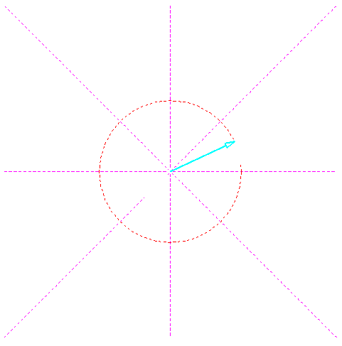
Right now the algorithm only works in octant 1 (the diagram is using regular coordinates instead of the upside coordinate system by screens which in turn is the vestigial remnant of old CRT monitors)
Lets consider the case where the slope is \(>1\) the algorithm is identical if we iterate over y instead of iterating over x, and we also need to change the second point of consideration from \((x_0 + 1, y_0)\) to \((x_0, y_0 + 1)\). Moreover the midpoint of the two points we have to choose from changes to \((x_0 + \frac12, y_0+1)\). All of these changes are immediately handled if we just swap the variables \(x_0\) and \(y_0\) and \(x_1\) and \(y_1\) and plot y, x instead of x, y since the variables are now inverted. Don’t take my word for it, try it and see.
plotLine(x0, y0, x1, y1)
	steep = false
	if abs(y1 - y0) > abs(x1 - x0):
		swap(x0, y0)
		swap(x1, y1)
		steep = true
    dx = x1 - x0
    dy = y1 - y0
    D = 2*dy - dx
    y = y0

    for x from x0 to x1
        plot(x, y)
        if D > 0
            y = y + 1
            D = D - 2*dx
        end if
        D = D + 2*dy
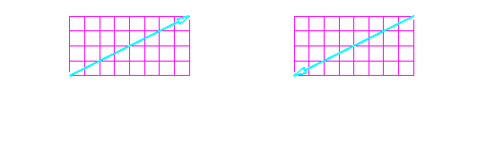
Now we have octant 1 and 2 done, what about octant 5 and 6. The above diagram shows us whats different between the two quadrants. Notice that the only difference in octant 5 and 6 is the direction in which our lines are being drawn, if we just swap the points whenever \(x_0 > x_1\) we get what we are looking for. Should we be doing this after or before the swap in case the slope is greater than 1? We should be doing this after we decide to swap variables for greater slopes. Because what we are doing right now is changing the order of the variables we are meant to be looping over, and the the swap for the loops is deciding which variable x or y we need to be looping over.
plotLine(x0, y0, x1, y1)
	steep = false
	if abs(y1 - y0) > abs(x1 - x0):
		swap(x0, y0)
		swap(x1, y1)
		steep = true
	if x0 > x1:
		swap(x0, x1)
		swap(y0, y1)
    dx = x1 - x0
    dy = y1 - y0
    D = 2*dy - dx
    y = y0

    for x from x0 to x1
        plot(x, y)
        if D > 0
            y = y + 1
            D = D - 2*dx
        end if
        D = D + 2*dy
What about cases when the slope is negative, which is what happens in octants 7 and 8? Going back to diagram with yellow and green dots this refers to the case where the line is sloping upwards and we now have to choose between the points \((x_0 + 1, y_0)\) and \((x_0 + 1, y_0 - 1)\) with the midpoint now being \((x_0+1, y_0 - \dfrac{1}{2})\) the difference function changes and if the value evaluated at this point is positive then we choose \((x_0 + 1, y_0 - 1)\). This can be fixed if we decrease the value of y instead of increase it and change the dy we use in the Difference equation to -dy.
plotLine(x0, y0, x1, y1)
	steep = false
	if abs(y1 - y0) > abs(x1 - x0):
		swap(x0, y0)
		swap(x1, y1)
		steep = true
	if x0 > x1:
		swap(x0, x1)
		swap(y0, y1)
    dx = x1 - x0
    dy = y1 - y0
    yi = 1
    if dy < 0:
	    yi = -1
	    dy = -dy
    D = 2*dy - dx
    y = y0

    for x from x0 to x1
        plot(x, y)
        if D > 0
            y = y + 1
            D = D - 2*dx
        end if
        D = D + 2*dy
The changes that we made to plot octants 5 and 6 still apply as its a valid operation for the entire left half of the plane and by making these changes octants 3 and 4 get covered on their own with no further changes.
In C++ everything we’ve done so far looks like this:
void line(int x0, int y0, int x1, int y1, TGAColor colour, TGAImage *image){
        // Bresenham Algorithm from Wikipedia (not exactly but pretty much the same)
        bool steep = false;
        if (std::abs(y1-y0)> std::abs(x1-x0)){
                std::swap(x0, y0);
                std::swap(x1, y1);
                steep = true;
        }
        if (x0 > x1) {
                std::swap(x0, x1);
                std::swap(y0, y1);
        }
        int yi = 1;
        int dx = x1 - x0;
        int dy = y1 - y0;
        if (dy < 0){
                yi = -1;
                dy = -dy;
        }
        int D =  2*dy - dx;
        int y = y0;

        for (int x = x0; x <= x1; x++){
                if(steep) image->set(y, x, colour);
                else image->set(x, y, colour);
                if (D > 0){
                        y += yi;
                        D -= 2*dx;
                }
                D += 2*dy;
        }
}
Wavefront OBJ File Format⌗
Anything following a hash character (#) is a comment.
An OBJ file may contain vertex data, free-form curve/surface attributes, elements, free-form curve/surface body statements, connectivity between free-form surfaces, grouping and display/render attribute information. The most common elements are geometric vertices, texture coordinates, vertex normals and polygonal faces:
# List of geometric vertices, with (x, y, z, [w]) coordinates, w is optional and defaults to 1.0.
v 0.123 0.234 0.345 1.0
v ...
...
# List of texture coordinates, in (u, [v, w]) coordinates, these will vary between 0 and 1. v, w are optional and default to 0.
vt 0.500 1 [0]
vt ...
...
# List of vertex normals in (x,y,z) form; normals might not be unit vectors.
vn 0.707 0.000 0.707
vn ...
...
# Parameter space vertices in (u, [v, w]) form; free form geometry statement (see below)
vp 0.310000 3.210000 2.100000
vp ...
...
# Polygonal face element (see below)
f 1 2 3
f 3/1 4/2 5/3
f 6/4/1 3/5/3 7/6/5
f 7//1 8//2 9//3
f ...
...
# Line element (see below)
l 5 8 1 2 4 9
Faces are defined using lists of vertex, texture and normal indices in the format vertex_index/texture_index/normal_index for which each index starts at 1 and increases corresponding to the order in which the referenced element was defined. Polygons such as quadrilaterals can be defined by using more than three indices.
Rendering a Wireframe⌗
As outlined by the Wavefront OBJ File Format we will have to read the array of vertices that have v as the first character in the line
v 0.437500 0.164063 0.765625
After which we can look at the array of faces that look like this
f 61/1/1 65/2/2 49/3/3
where the first number in the blocks separated by spaces refer to the index of the vertex that makes up that face, in this case, vertex number 61, 65 and 49 make up this face, (.obj files begin indexing from 1 so we should look at index 60, 64 and 48 in our array).
Writing a basic parser⌗
The first thing we’ll do is define a struct vec3 with some usual mathematical operations to represent the vertices as they are actual vectors in 3D space and we might want to do some regular vector maths with them.
struct Vec3 {
	// A vector is just a struct of three floats
	struct {float x, y, z;};
	// with default value 0
	Vec3() : x(0), y(0), z(0) {}
	Vec3(float _x, float _y, float _z) : x(_x),y(_y),z(_z) {}

	// defining a cross product
	inline Vec3 operator ^(const Vec3 &v) const { return Vec3(y*v.z-z*v.y, z*v.x-x*v.z, x*v.y-y*v.x); }
	// dot product
	inline float operator *(const Vec3 &v) const { return x*v.x + y*v.y + z*v.z; }
	// vector addition
	inline Vec3 operator +(const Vec3 &v) const { return Vec3(x+v.x, y+v.y, z+v.z); }
	// vector subtraction
	inline Vec3 operator -(const Vec3 &v) const { return Vec3(x-v.x, y-v.y, z-v.z); }
	// scalar multiplication
	inline Vec3 operator *(float f) const { return Vec3(x*f, y*f, z*f); }
	// length of the vector
	float norm () const { return std::sqrt(x*x+y*y+z*z); }
	// normalising a vector
	Vec3 &normalize(float l=1) { *this = (*this)*(l/norm()); return *this; }

	// A way to display the vector
	friend std::ostream& operator<<(std::ostream& s, Vec3 v){
		s << "(" << v.x << ", "<< v.y << ", "<< v.z << ")\n";
		return s;
	}
};
All right, now that we have vector like we are used to in mathematics we can move on to representing models.
class Model {
private:
	// all the vertices of the model
	std::vector<Vec3> verts_;
	// faces are not limited to three vertices btw, which is we use vectors
	std::vector<std::vector<int>> faces_;
public:
	Model(const char *filename);
	~Model();
	// number of vertices and faces
	int nverts();
	int nfaces();
	// ways to access a vertex by index
	Vec3 vert(int i);
	// ways to access a face by index
	std::vector<int> face(int idx);
};
Now we need a program a way to construct this model and define all the methods we’ve declared here.
Model::Model(const char *filename): verts_(), faces_(){
        // constructing the model object
        std::ifstream in;
        in.open(filename);
        if (in.fail()) return;
        std::string line;

        while (!in.eof()){
                std::getline(in, line);
                std::istringstream iss(line.c_str());
                char trash;
                if (!line.compare(0, 2, "v ")){
                        // throwing away the 'v ' part
                        iss >> trash;
                        Vec3 v;
                        for (int i=0; i<3; i++) iss>>v.raw[i];
                        verts_.push_back(v);
                } else if (!line.compare(0, 2, "f ")) {
                        std::vector<int> f;
                        int itrash, idx;
                        iss >> trash;
                        // taking the first value and throwing away the remaining 2 indices
                        // we are assuming that there will always be groups of three numbers
                        // separated by / but the obj format allows those to be omitted
                        // so this is not particularly good
                        while (iss >> idx >> trash >> itrash >> trash >> itrash){
                                idx--; // .obj indexing starts at 1
                                f.push_back(idx);
                        }
                        faces_.push_back(f);
                }
        }
}

Model::~Model() {
}

int Model::nverts() {
    return (int)verts_.size();
}

int Model::nfaces() {
    return (int)faces_.size();
}

std::vector<int> Model::face(int idx) {
    return faces_[idx];
}

Vec3 Model::vert(int i) {
    return verts_[i];
}
Now we have a way to read wireframes.
Rendering⌗
int main(int argc, char** argv) {
        int width = 500, height = 500;
        TGAImage image(width, height, TGAImage::RGB);
        Model monke("./suzanne.obj");
        for (int i=0; i < monke.nfaces(); i++) {
                std::vector<int> face = monke.face(i);
                for (int j=0; j < 3; j++){
                        Vec3 v0 = monke.vert(face[j]);
                        Vec3 v1 = monke.vert(face[(j+1)%3]);
                        int x0 = (v0.x+1.)*width/2.;
                        int y0 = (v0.y+1.)*height/2.;
                        int x1 = (v1.x+1.)*width/2.;
                        int y1 = (v1.y+1.)*height/2.;
                        line(x0, y0, x1, y1, white, &image);
                }
        }
        image.write_tga_file("output.tga");
        return 0;
}
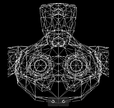
This is extremely straightforward so I am not gonna bother explaining whats going on in detail, it just connects the line and draws them using Bresenham’s Line Drawing Algorithm.
Suzanne is upside down, but that is because while .obj uses coordinates that are the right way up, the coordinate system of displays is upside down.
Moreover, since we are completely ignoring the z value of the vector we are effectively looking at a shadow of Suzanne orthographic projection that is cast from a light source at infinity.
The image looks funky as hell, there are clearly too many lines and we are rendering too much of the scene, we can make this better by discarding the faces that are pointing away from the camera.
ssloy/tinyrenderer uses z-buffers in the next few lessons, but I am not there yet and I want to use simple normal vector based culling right now and look at Suzanne in all her glory.
The idea is to find a normal vector of the triangle, and then the dot product with the camera vector should be positive is the normal is lying along it
int main(int argc, char** argv) {
        int width = 500, height = 500;
        TGAImage image(width, height, TGAImage::RGB);
        Model monke("./suzanne.obj");
        Vec3 camera{0, 0, -1};
        for (int i=0; i < monke.nfaces(); i++) {
                std::vector<int> face = monke.face(i);
                // deciding if it should be drawn or not
                Vec3 normal = (monke.vert(face[1]![[Suzanne1.jpeg]]) - monke.vert(face[0])) ^ (monke.vert(face[2]) - monke.vert(face[0]));
                if (camera*normal >= 0) continue;
                for (int j=0; j < 3; j++){
                        Vec3 v0 = monke.vert(face[j]);
                        Vec3 v1 = monke.vert(face[(j+1)%3]);
                        int x0 = (v0.x+1.)*width/2.;
                        int y0 = (v0.y+1.)*height/2.;
                        int x1 = (v1.x+1.)*width/2.;
                        int y1 = (v1.y+1.)*height/2.;
                        line(x0, y0, x1, y1, white, &image);
                }
        }
        image.write_tga_file("output.tga");
        return 0;
}
Better.
Line Sweeping Triangle Rasterisation⌗
We need to colour the triangle by drawing horizontal lines from one side of the triangle to the other. But how do we decide which side we need to start from.
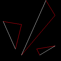
Its pretty clear that when we do this horizontal line sweeping there is one line that is drawn towards or from, in the image above we want horizontal lines to either start at the white lines of in the case of the smallest triangle end at the white line.
By looking at it is clear that the white line is the one which has the maximum y “component”. And to find that, basic bubble sort is sufficient.
void triangle(Vec3 p0, Vec3 p1, Vec3 p2, TGAColor colour, TGAImage *image){
        // sorting the points based on y coordinate
        if (p0.y > p1.y) std::swap(p0, p1);
        if (p1.y > p2.y) std::swap(p1, p2);
        if (p0.y > p1.y) std::swap(p0, p1);

        line(p0, p1, colour, image);
        line(p1, p2, colour, image);
        line(p2, p0, white, image);
}
Colouring the triangle⌗
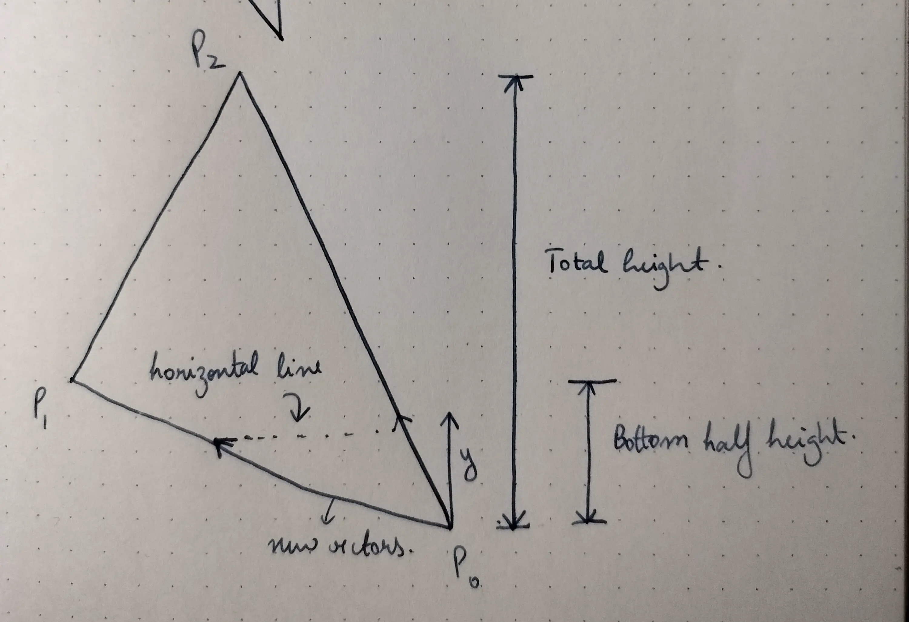
Consider the lower half of the triangle, we will be drawing horizontal lines that start from one of the lines and end at the other, and its much easier to do this when we think in terms of vectors, the diagram below is very self explanatory, we are merely scaling the vectors along those lines by how far up we go.
void triangle(Vec3 p0, Vec3 p1, Vec3 p2, TGAColor colour, TGAImage *image){
        // sorting the points based on y coordinate
        if (p0.y > p1.y) std::swap(p0, p1);
        if (p1.y > p2.y) std::swap(p1, p2);
        if (p0.y > p1.y) std::swap(p0, p1);

        // line(p0, p1, colour, image);
        // line(p1, p2, colour, image);
        // line(p2, p0, white, image);

        int height = p2.y - p0.y;  // used to scale the vector along p0->p2
        int bottom_half_height = p1.y - p0.y;  // used to scale the vector along p0->p1

        for (int y = p0.y; y <= p1.y; y++){
                // the x value for the line joining p0 and p1
                float scaler_02 = (y - p0.y) / height;
                float scaler_01 = (y - p0.y) / bottom_half_height;
                Vec3 vec_02 = p0 + (p2 -  p0) * scaler_02;
                Vec3 vec_01 = p0 + (p1 -  p0) * scaler_01;
                if (vec_01.x > vec_02.x) std::swap(vec_01, vec_02);
                for (int x = vec_01.x; x <= vec_02.x; x++){
                        image->set(x, y, white);
                }
        }
}
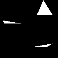
I know I said bottom half, and this is the top half, I just didn’t bother flipping the y-axis, display nonsense (maybe at this point I should just invert the y-axis while rendering).
And we can do something similar for the top half
void triangle(Vec3 p0, Vec3 p1, Vec3 p2, TGAColor colour, TGAImage *image){
        // sorting the points based on y coordinate
        if (p0.y > p1.y) std::swap(p0, p1);
        if (p1.y > p2.y) std::swap(p1, p2);
        if (p0.y > p1.y) std::swap(p0, p1);

        // line(p0, p1, colour, image);
        // line(p1, p2, colour, image);
        // line(p2, p0, white, image);

        int height = p2.y - p0.y;  // used to scale the vector along p0->p2
        int bottom_half_height = p1.y - p0.y;  // used to scale the vector along p0->p1

        for (int y = p0.y; y <= p1.y; y++){
                // the x value for the line joining p0 and p1
                float scaler_02 = (y - p0.y) / height;
                float scaler_01 = (y - p0.y) / bottom_half_height;
                Vec3 vec_02 = p0 + (p2 -  p0) * scaler_02;
                Vec3 vec_01 = p0 + (p1 -  p0) * scaler_01;
                if (vec_01.x > vec_02.x) std::swap(vec_01, vec_02);
                for (int x = vec_01.x; x <= vec_02.x; x++){
                        image->set(x, y, white);
                }
        }

        // top half
        int top_half_height = p2.y - p1.y;  // used to scale the vector along p1->p2
        for (int y = p1.y; y <= p2.y; y++){
                float scaler_02 = (y - p0.y) / height;
                float scaler_12= (y - p1.y) / top_half_height;
                Vec3 vec_02 = p0 + (p2 -  p0) * scaler_02;
                Vec3 vec_12 = p1 + (p2 -  p1) * scaler_12;
                if (vec_12.x > vec_02.x) std::swap(vec_12, vec_02);
                for (int x = vec_12.x; x <= vec_02.x; x++){
                        image->set(x, y, white);
                }
        }
}